When you have completed the steps described in Preparations you can build an instrumented version of your application. When the instrumented application runs, coverage information will be collected and you can later view it either in a table or graphically in state chart diagrams.
When you have configured a TC for instrumentation you can build it as usual. You will notice that it takes slightly longer, and that there are printouts in the console showing that the generated code is instrumented before it's built.
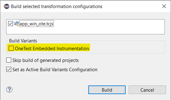
If you chose not to change your TC when you configured it for instrumentation, you will be prompted when the TC is built:
If the "OneTest Embedded Instrumentation" checkbox is checked, an instrumented version of the application will be built. Otherwise a regular version of the application will be built.
An instrumented application behaves exactly like a non-instrumented application at run-time, except that it runs somewhat slower since run-time data gets collected. This means that you can run an instrumented application in the same ways as you normally would run your application. For example, you can run it from the command-line, from the Model RealTime user interface, or from the model debugger. You can also execute your normal test suites which may run the application one or several times.
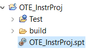
The collected run-time data is saved to an .spt file inside the instrumentation project. By default this happens when the application terminates, but there are settings on the instrumentation project to force it to be saved earlier than that. For example, it can be saved after a certain number of instrumented functions have been called or the first time you press Ctrl+C when running the application from the command line. Refer to the OneTest Embedded documentation to learn more about this.
To make the generated .spt file visible in the instrumentation project you can perform the Refresh command on the instrumentation project:
Right-click on the .spt file and invoke the command Create Application Result. OneTest Embedded will then process the .spt file and generate an application result file from it. You can see this file under the "Application Result" folder in the instrumentation project:
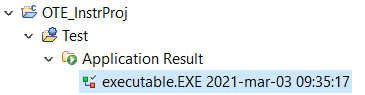
The application result file name is constructed from the name of the instrumented executable and a timestamp (the time the application result file was created). To avoid confusion you should avoid reusing the same instrumentation project for different TCs, at least if they build applications with the same name.
The application result file is an archive that contains all run-time data that the OneTest Embedded instrumentation has collected. One part of this run-time data is the model coverage information. It consists of an .mcov file that contains information about all states and transitions that have executed, and how many times they executed.
To view the coverage data for the execution, double-click either the application result file or an .mcov file. This opens the Model Coverage Viewer which shows the coverage data in a tabular view.
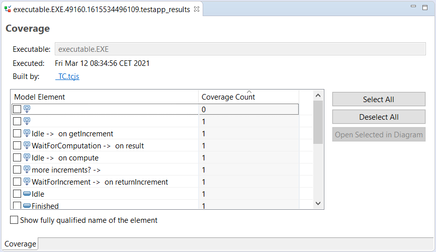
In the Coverage table you can see each model element (i.e. states and transitions) and how many times they have executed. By sorting the table on the "Coverage Count" column you can easily find those parts of the state machines that were not executed. In the above picture we see that there is one transition that never executed.
Use the context menu on the model elements in the Coverage table to navigate to them.
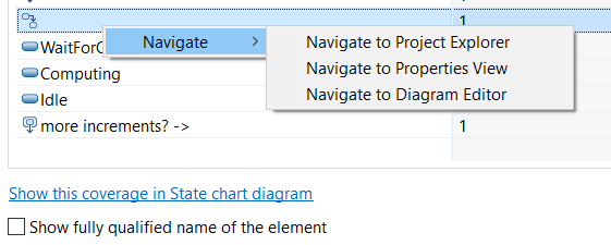
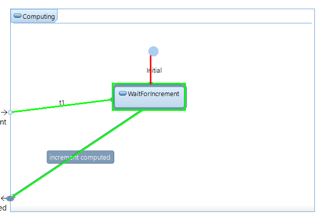
You can also show the coverage graphically in state chart diagrams. Click the hyperlink Show this coverage in State chart diagram at the bottom of the Model Coverage Viewer. It will open all state chart diagrams showing the listed model elements, and highlight in each diagram which states and transitions that were never executed (in red color) and those that were executed at least once (in green color). Here is an example:
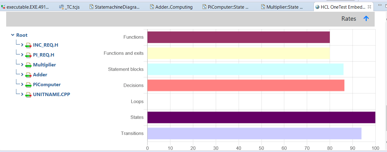
Finally, you can show the coverage in an HTML report which also will contain the coverage computed at code-level. Right-click on an application result file and perform the command Open With - HTML Reports - Coverage.
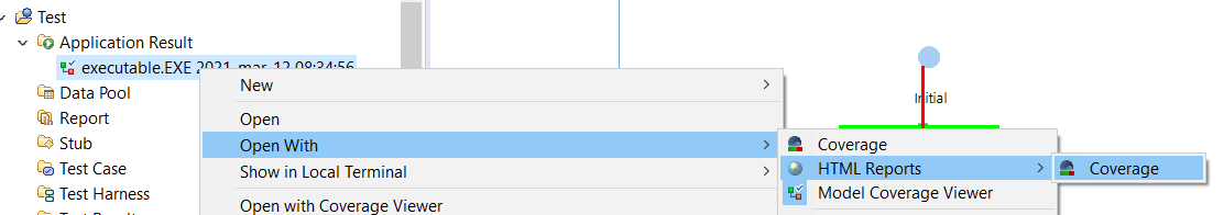
An interactive HTML page will open where you can explore the coverage both for code and state machines.